1. Adsorption Basics and Reactive Transport [September 2024]
Methodology
This study is based on numerical resolution of the advection-diffusion-reaction equation using finite differences and finite elements (Python/FEniCS).
Fundamental Transport Equation with Adsorption
Contaminant transport in porous media (filter) is governed by:
where the source term γ represents adsorption/desorption on the filter substrate:
with:
- θ: filter porosity
- ρ_s: filter density
- K_d: partition coefficient (adsorption)
Scaling and Retardation Factor
The equation can be rewritten as a classical advection-diffusion equation with effective coefficients:
The retardation factor R > 1 represents the slowing down of the concentration front due to adsorption: higher R means more effective contaminant retention.
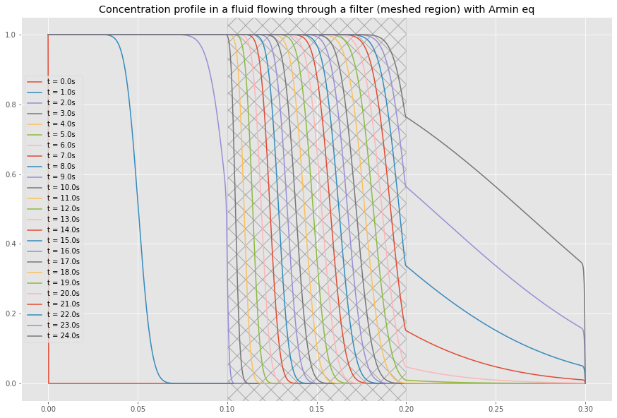
Profil de concentration dans le filtre - Solution numérique de l'équation d'advection-diffusion-réaction
Complete Adsorption-Diffusion Model
The full system consists of the fluid and filter domains considered as a coupled system in which concentrations in fluid (c_ℓ) and filter (c_f) are considered. The reduction of the fluid concentration corresponds to the loading of the filter (or simply to the adsorption of compounds by the filter, whose concentration increases.
This model integrates:
- α: contaminant adsorption coefficient on filter
- κ: filter-to-fluid diffusion coefficient (desorption)
- ε: saturation factor (adsorption dependence on filter loading)
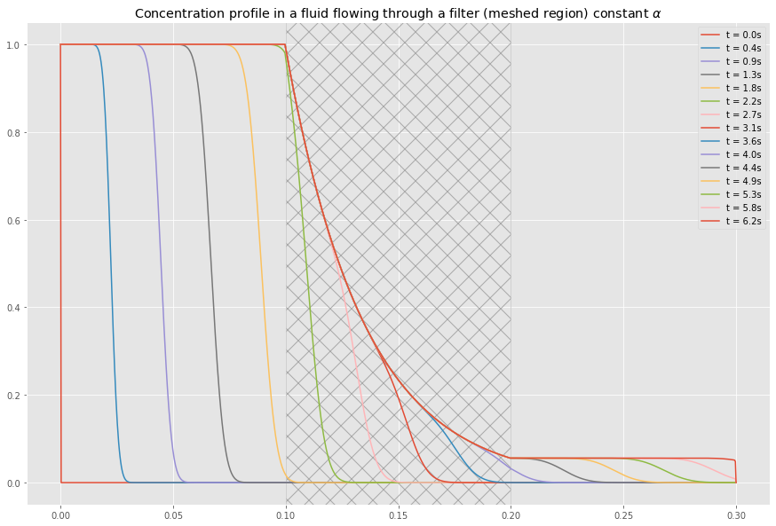
Évolution temporelle de la concentration adsorbée sur le substrat du filtre
Special Case: Variable Adsorption Coefficient
As the filter loads, adsorption efficiency decreases. The effective adsorption coefficient α(t) decreases with increasing filter loading c_f.
This nonlinearity leads to progressive filter saturation and contaminant breakthrough.
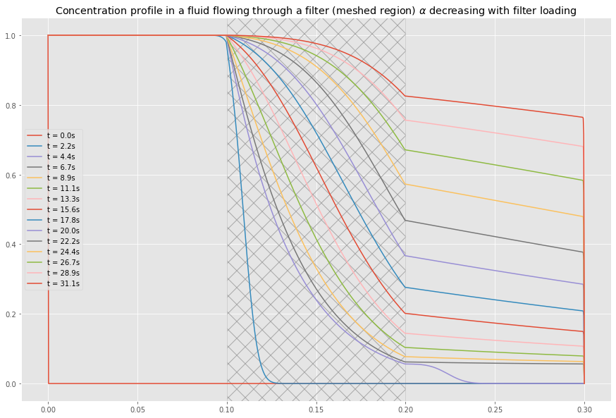
Modèle non-linéaire : décroissance du coefficient d'adsorption avec le chargement du filtre. La concentration de sortie augmente.
Physical Interpretation
- Retardation factor R: quantifies contaminant slowing in filter
- Initial efficiency: near 100% while c_f ≪ maximum capacity
- Breakthrough: contaminant appears at outlet when filter saturates
- Langmuir model: possible extension with nonlinear adsorption isotherm
2. Contaminant Migration from Tubing [November 2024]
This section presents simulation of substance migration from polymer tube wall to flowing fluid.
Geometric Configuration
- Inner diameter: 4 mm
- Wall thickness: 0.6 mm
- Length: 1 m
- Flow rate: 100 mL/h
- Inner volume: 12.57 mL
Substance Properties
Two substances with contrasting diffusivities are simulated:
Migration Parameters
- Substance 1: Dₛ = 10⁻⁶ mm²/s, Dℓ = 5×10⁻⁴ mm²/s, μ = 72 μg/g
- Substance 2: Dₛ = 5×10⁻⁶ mm²/s, Dℓ = 2×10⁻³ mm²/s, μ = 252 μg/g
- Partition coefficient: F = 10 (solid concentration / fluid concentration at equilibrium)
Pure Diffusion Regime
Without flow, migration is governed by Fick's second law:
After 1 hour of diffusion, fluid concentrations reach:
- Substance 1: 0.0408 mg in inner volume (12.57 mL)
- Substance 2: 0.2420 mg

Migration par diffusion pure : profil de concentration après 1 heure.
Advection-Diffusion Regime
With flow, the transport equation becomes:
where velocity profile v is solution of Navier-Stokes equations:
For a flow rate of 100 mL/h (bulk velocity ≈ 2.21 mm/s), Reynolds number is very low (Re ≪ 1), flow is laminar with parabolic profile (Poiseuille).

Migration avec écoulement : profil de concentration à t = 2 heures
Results for Continuous Flow
For a total flowed volume of 400 mL (duration: 4 hours), cumulative contaminant masses are:
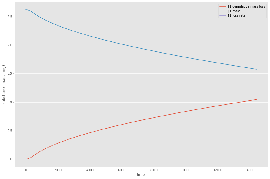
Masse cumulée de contaminants dans le fluide en fonction du volume écoulé
Flow Rate Profile Impact
Three scenarios compared for same total volume (400 mL):
Scenario A - Continuous
Constant flow 100 mL/h
m₂ = 1.044 mg
Duration: 4h00
Scenario B - Interrupted
100 mL/h (1.5h) → stop 1h → resume
m₂ = 1.150 mg (+10%)
Duration: 5h00
Scenario C - Slowed
100 mL/h (1.5h) → stop 1h → 50 mL/h
m₂ = 1.427 mg (+37%)
Duration: 7h30
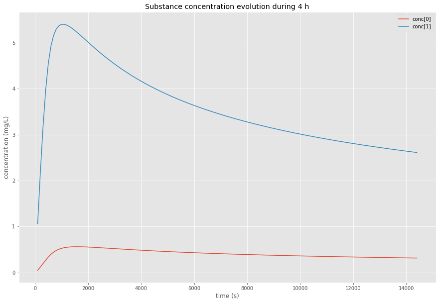
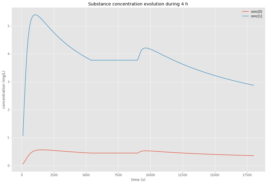
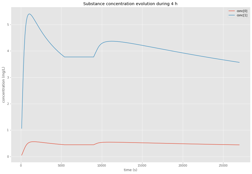
Trois scénarios de débit : continu, interrompu, interrompu avec réduction de vitesse
Interpretation: Interruptions and slowdowns significantly increase migration due to prolonged contact time between fluid and tube wall. Continuous processing minimizes contamination.
3. Advanced Filtration System Modeling [December 2024]
Steady State and Beer-Lambert Law
In steady state, neglecting diffusion from filter (κ ≈ 0), the system reduces to:
whose solution is an exponential decay:
This relationship, analogous to Beer-Lambert law in optical absorption, characterizes contaminant attenuation in the filter.
Décroissance exponentielle de la concentration dans le filtre (zone hachurée) pour une adsorption constante.
Breakthrough Curve
The key parameter for filter sizing is the breakthrough curve: outlet concentration evolution as function of time or treated volume.
[Simulation] Courbe de percée (breakthrough)
Concentration en sortie de filtre vs temps
Évolution de la concentration en sortie de filtre - saturation progressive du média filtrant
Optimal Filtration Parameters
Filtration system optimization relies on trade-off between:
- Efficiency: contaminant retention capacity (high α, high R)
- Lifetime: volume treated before breakthrough (filter capacity)
- Pressure drop: impact on flow rate (Darcy's law, Navier-Stokes in porous media)
with K the porous medium permeability (m²), function of porosity and pore size.
4. Coupled System: Tube + Filter [December 2024]
The complete model integrates:
- Migration: diffusion from tube wall + advection by flow
- Filtration: contaminant adsorption on filter media
- Coupling: filter inlet concentration = tube outlet concentration
[Simulation] Système couplé : tube + filtre
Concentration entrée: 0.125 mg/L · Efficacité filtration: 92%
Modèle complet : migration depuis les parois du tube suivie d'une filtration
Case Study
Consider a system where:
- Fluid flows through 1 m tubing (wall migration)
- Then through 10 cm thick filter (adsorption)
- Flow rate: 100 mL/h
- Substance 1 (previous parameters)
Simulation Results
Sensitivity Analysis
Coupled system efficiency depends on several parameters:
Parameter: Filter thickness
Exponential law
Parameter: Flow rate
Contact time
Parameter: Tube migration
Diffusivity dependence
[Simulation] Comparaison des scénarios
Masse migrée: +12% (interruption), +41% (ralentissement)
Impact du profil de débit sur la masse totale de contaminants migrés
Conclusion and Perspectives
Numerical simulation of coupled migration and filtration phenomena enables:
- Quantification of actual product contamination based on process parameters
- Optimization of filtration system sizing (thickness, porosity, flow rate)
- Anticipation of filter saturation and replacement scheduling
- Comparison of different production scenarios (continuous vs batch)
Industrial Applications:
- Pharmaceutical: API purification, extractables & leachables control
- Food & Beverage: beverage filtration, packaging material validation
- Environmental: water treatment, permeable reactive barriers
- Chemical: continuous separation and purification