1. Anharmonic Oscillator
Introduction
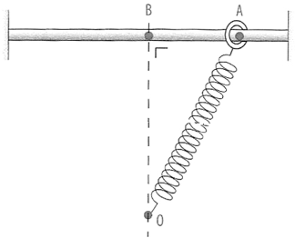
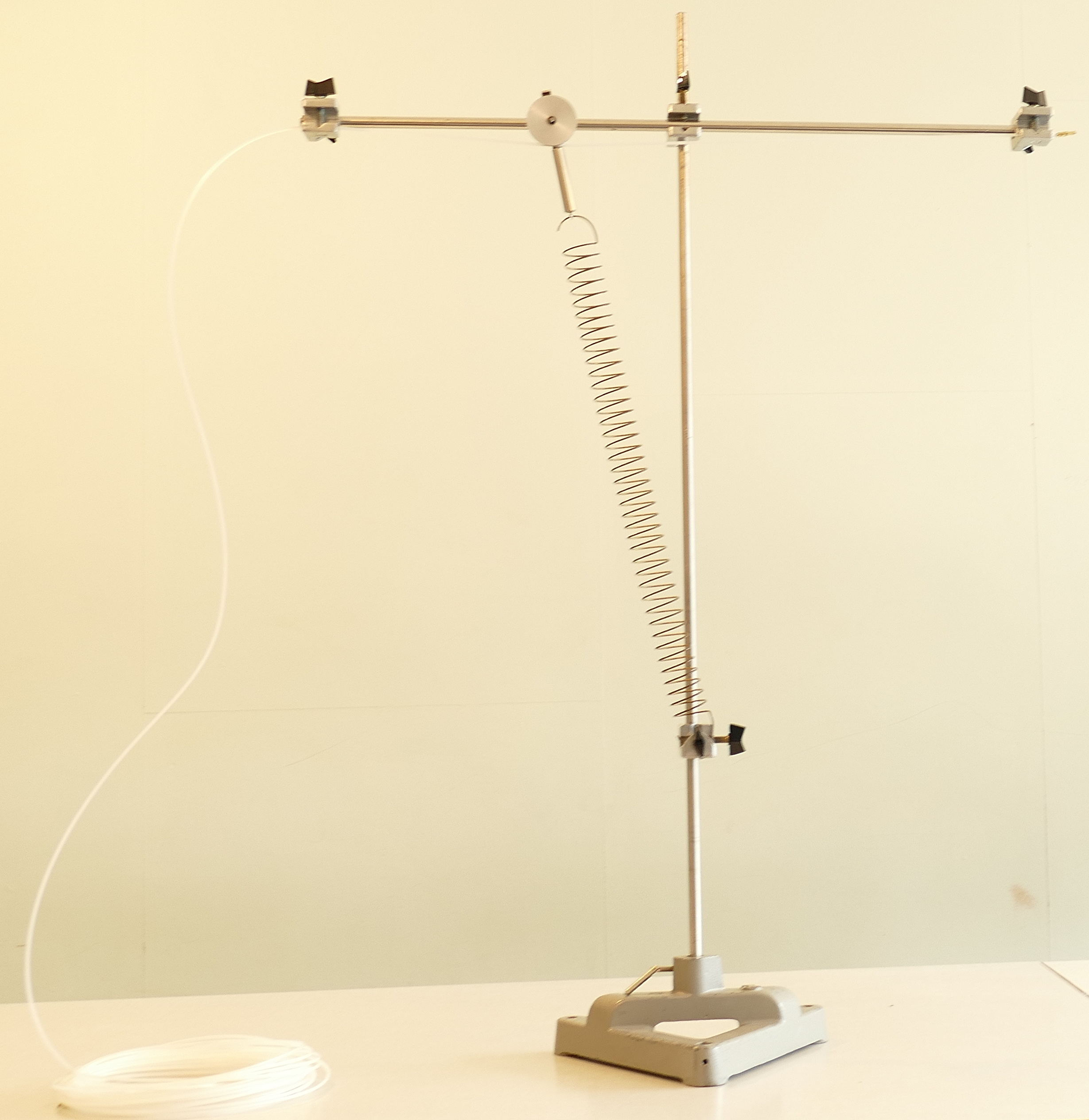
This project is born out of a laboratory manipulation with a wagon on a rail. The wagon is bound to a fixed point under the rail
with a spring. As the wagon is pushed out of its equilibrium position (which is an extend zone because of the mechanical friction)
it oscillates and slows down. The oscillation amplitudes decreases with time.
Although this mechanical system is rather simple it gives rise to an analytical problem which is quite complex in the form of an anharmonic
oscillator of degree 3. Evidently the degree 3 is quite arbitrary and depends where we stop the series expansion of the square root (see below).
The initial objective was to look at the corrections of the linear term that express qualitatively the numerical solution of the full problem.
Historically, in 1923, when Werner Heisenberg worked to discover the fundamental laws of quantum mechanics, he got interested in exactly this same
problem. Later on, as this precise problem involves terms of opposite parity, he decided for another problem without the even term (cf.
Jagdish Mehra, The Historical Developpment of Quantum Theory) that he expanded in Fourier series. This new problem led him to discover
the famous commutation relations that bear his name and that are at the foundation of the quantization rule of quantum mechanics.
In our problem, the motion equation reads
$$
\frac{d^2}{dt^2}x=-\omega_0\left(1-\frac{\ell_0}{\sqrt{d^2+x^2}}\right)\,(x+\mu\, d\, \mathrm{sign}(\frac{d}{dt} x))
$$
In this relation, the fraction with the square root can be expanded, and the problem reduces to
$$
\frac{d^2}{dt^2}z=-\omega_0^2 z+\alpha z^2 -\beta z^3
$$
where \(\omega_0^2=\frac km\), \(d=OA\) and \(\ell_0\) is the rest length of the spring, and \(z=\frac xd\).
The term in \(z^2\) breaks the parity symmetry and is the one that Heisenberg got rid of in his quest for quantum mechanics.
Solution
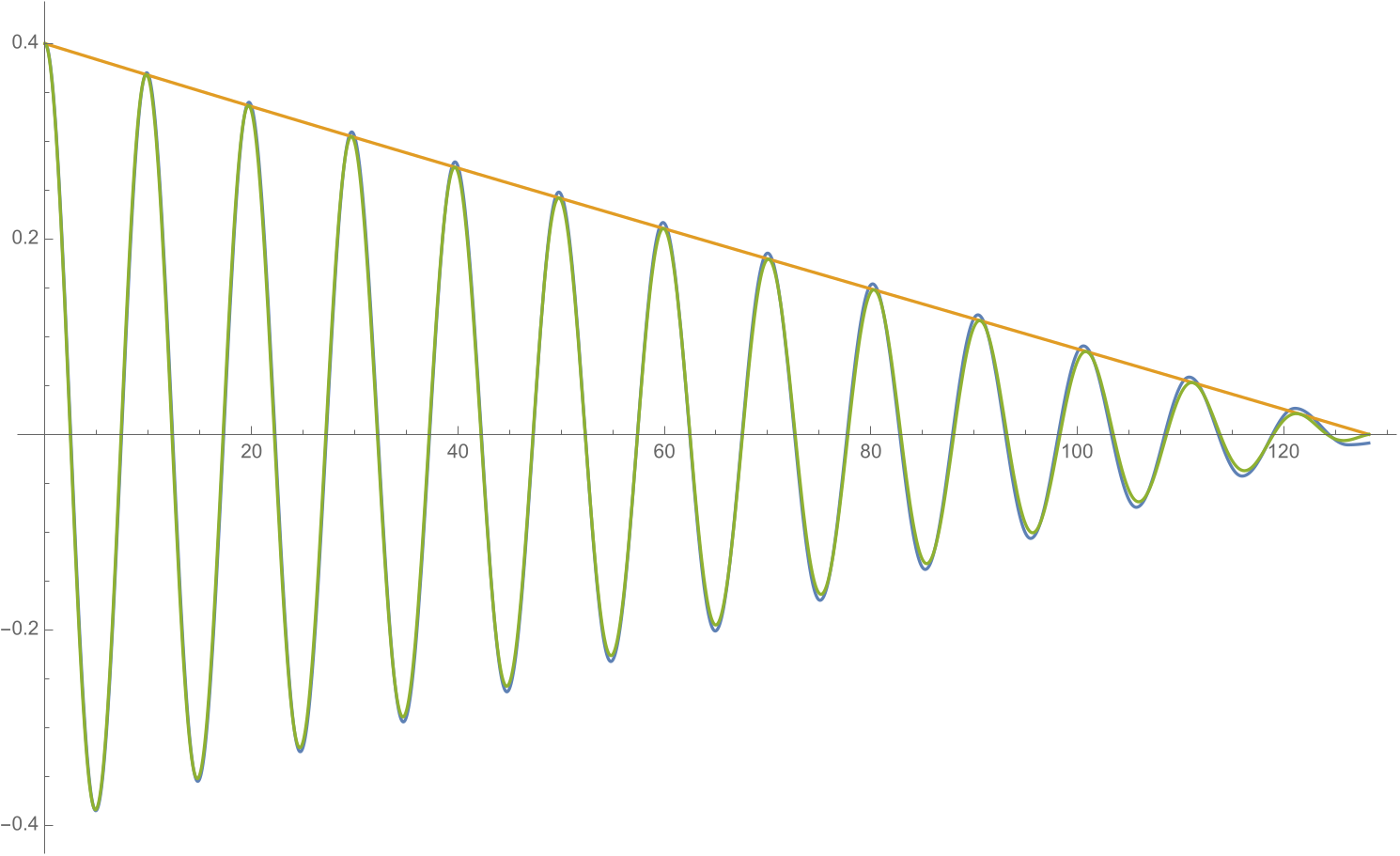
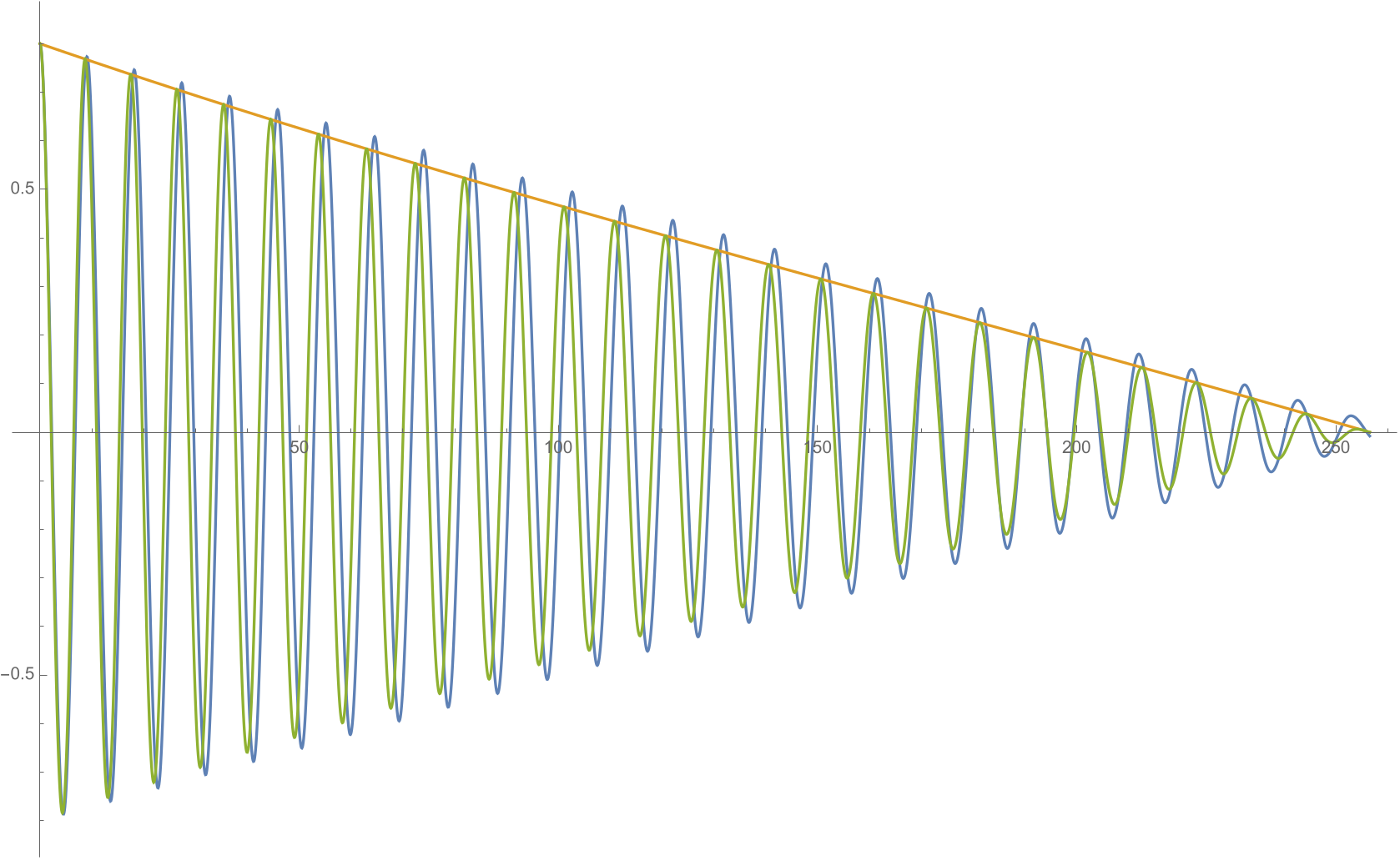
The number of oscillations for an initial amplitude \(z_0\) can be expressed as $$ n=\frac {z_0}{4\mu} $$
The following graphs compare the full numerical solution (in blue) with the solution containing the expansion terms up to degree 3 (green). The left graph picture the situation for medium initial amplitude \(z_0=0.4\) and the right one for a large amplitude \(z_0=0.8\).