1. The Basic SIR Model [February 2025]
Methodology
This study presents a comprehensive analysis of the SIR model (Susceptible-Infectious-Removed) with numerical resolution of differential equations and nullcline analysis.
The Three Compartments
The classic SIR model divides the population into three compartments:
- S (Susceptible): non-immune individuals who can be contaminated
- I (Infectious): disease carriers who contaminate susceptibles
- R (Removed): immune (after recovery) or deceased
where N is the total population, and N_S, N_I, N_R are the sizes of each compartment.
Model Equations
Disease transmission is modeled by a mass action term:
where β is the transmission rate. The force of infection is defined as λ = β I.
Let τ be the infectious period, then the recovery rate is γ = 1/τ.
with:
- μ: birth rate
- δ: death rate (often δ = μ for constant population)
- γ: recovery rate
- β: transmission rate
Basic Reproduction Number R₀
An infectious individual contaminates on average β people per time unit during a period τ:
This fundamental parameter determines epidemic behavior:
- R₀ < 1: epidemic dies out
- R₀ > 1: epidemic spreads
- R₀ = 1: critical threshold
Impact du nombre de reproduction de base R₀ sur la sévérité de l'épidémie
_beta.0.7_gamma.0.2_mu.0.png)
Évolution temporelle des trois compartiments : Susceptibles (S), Infectés (I), Retirés (R)
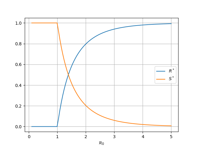
When the epidemic starts, the fraction of infected I(t) grows exponentially with an initial growth rate given by r = γ (R₀ - 1). The higher R₀, the faster the initial growth and the more severe the epidemic. For typical R₀ values (2 to 3 for influenza, 3 to 5 for COVID-19), we observe a rapid growth in the number of infected, highlighting the importance of control measures to reduce R₀ below 1. We also note that the final fraction of the population affected by the epidemic (R*) is an increasing function of R₀, with a rapid transition around R₀ = 1. This fraction does not necessarily equal 1 even for high R₀ values, due to herd immunity that develops as individuals move into the R compartment. When the number of susceptibles S(t) falls below the critical threshold 1/R₀, the growth of I(t) slows down and eventually declines, even if R₀ > 1. This explains the characteristic bell-shaped curve of the epidemic: rapid growth followed by a gradual decline as herd immunity develops.
2. Nullclines and Stationary Points [February 2025]
Nullclines
Nullclines are curves where derivatives vanish. For the SIR model with δ = μ:
I nullcline (dI/dt = 0):
S nullcline (dS/dt = 0):
_beta.0.7_gamma.0.2_mu.0.png)
Portrait de phase S-I : évolution de la fraction d'infectés en fonction des susceptibles
Stationary Points
Two types of fixed points:
- Disease-free fixed point: (S*, I*, R*) = (1, 0, 0) (or adapted according to μ, δ)
- Endemic fixed point: (S*, I*, R*) with I* > 0 (appears when R₀ > 1)
_beta.0.7_gamma.0.2_mu.0.png)
Champ de vecteurs montrant la direction de l'évolution du système
Nullcline Interpretation
- Nullcline intersection gives equilibrium points
- I nullcline is vertical: critical susceptible threshold
- Below threshold (S < S_nc), I decreases
- Above threshold (S > S_nc), I increases (if I > 0)
3. SIR Model without Birth/Death [February 2025]
Without population dynamics (μ = δ = 0), the model simplifies:
Proliferation Condition
For disease spread, we need dI/dt > 0:
The disease can only proliferate if the susceptible fraction is high enough.
Implicit S-R Relation
Dividing the S equation by the R equation:
This equation is readily solved:
with S(0) = 1 (initially, no one is immune).
_beta.0.7_gamma.0.2_mu.0.png)
Relation implicite entre susceptibles et retirés : S = exp(-R₀·R)
Stationary Solution
At equilibrium (t → ∞), I* = 0 and S* + R* = 1, giving the implicit equation:
Solving this equation gives the final fraction of the population affected by the epidemic.

Fraction finale de la population touchée par l'épidémie en fonction de R₀
Numerical Example
- R₀ = 3.5
- τ = 5 days → γ = 0.2 day⁻¹
- β = R₀ × γ = 0.7 day⁻¹
- Stationary state: S* = 0.034, I* = 0, R* = 0.966
- Interpretation: 96.6% of the population will be affected
_beta.0.7_gamma.0.2_mu.0.png)
Trajectoire du système dans le plan infectés-retirés
4. SIR Model with Birth and Death [February 2025]
Introducing population dynamics (μ > 0, δ = μ) maintains constant total population but allows susceptible renewal through births.
Parameters
- R₀ = 3.5
- γ = 0.2 day⁻¹ (τ = 5 days)
- β = 0.7 day⁻¹
- μ = δ = 0.02 day⁻¹ (birth/death rate)
New Endemic Fixed Point
Unlike the case without birth/death, the system converges to an endemic fixed point with I* > 0:
_beta.0.7_gamma.0.2_mu.0.02.png)
Modèle avec dynamique de population : apparition d'un point fixe endémique non nul
Behavior Comparison
Without birth/death
Disease extinction
With birth/death
Stable endemic state
Births maintain a constant flow of new susceptibles, allowing the disease to persist in the population. This is typical of endemic diseases like seasonal influenza.
Numerical Verification
After simulation up to t = 200 days, values converge to the theoretical fixed point:
5. Conclusion and Perspectives [February 2025]
Key Results
SIR model analysis highlights several fundamental results in mathematical epidemiology:
- Epidemic threshold: R₀ > 1 is necessary for epidemic spread
- Herd immunity: when susceptible fraction drops below 1/R₀, epidemic recedes
- Final size: given by implicit equation 1 - exp(-R₀ R*) - R* = 0
- Endemicity: with population renewal, disease can persist indefinitely
Model Extensions
The basic SIR model can be enriched for more complex situations:
SEIR
Adds E (Exposed) compartment for incubation period
SIRS
Immunity loss: recovered return to susceptible compartment
Age-structured
Age-dependent contact and mortality rates
Spatial mobility
Geographic disease spread (meta-population models)
Practical Applications
These models are used daily by public health agencies for:
- Forecasting epidemic evolution (influenza, COVID-19, Ebola...)
- Evaluating control measures impact (lockdown, vaccination)
- Optimizing resource allocation (hospital beds, vaccines)
- Determining vaccination thresholds for herd immunity